

Why This Issues, by Stakeholder
- Customers and dapp builders. Decrease common handover latency means much less idle time between leaders, and thus extra slots per unit of wall-clock time. This may increasingly have an effect on transaction senders, who shouldn’t assume that consecutive leaders are geographically unbiased.
- Validators. Validators in sparse areas profit most, as they’re much extra more likely to have a close-by predecessor than at the moment. The variety of chief home windows a validator will get in an epoch is unchanged, solely their respective order adjustments.
- Core contributors. The chief schedule computation turns into extra advanced and is dependent upon reported areas.
TL;DR
- Geo-aware chief schedule is promising to enhance handoff latency, lowering stress for stake focus in macroregions
- This evaluation exhibits that the
STAKE_FLOORparameter (denoted with right here) ought to keep round 10%- Larger values make the fake-location assault costlier, however above 10%, Asia (about 10.4% of stake at the moment) loses native bins
- For the
RUN_LENGTHparameter (denoted with right here) shouldn’t go above 7- It is dependent upon which danger we wish to reduce, and ranges between 3 and seven
- When coalitions are thought-about, if we repair , our simulation framework suggests a restricted absolute improve in MEV-opportunity rising from consecutive chief home windows
Related Charts
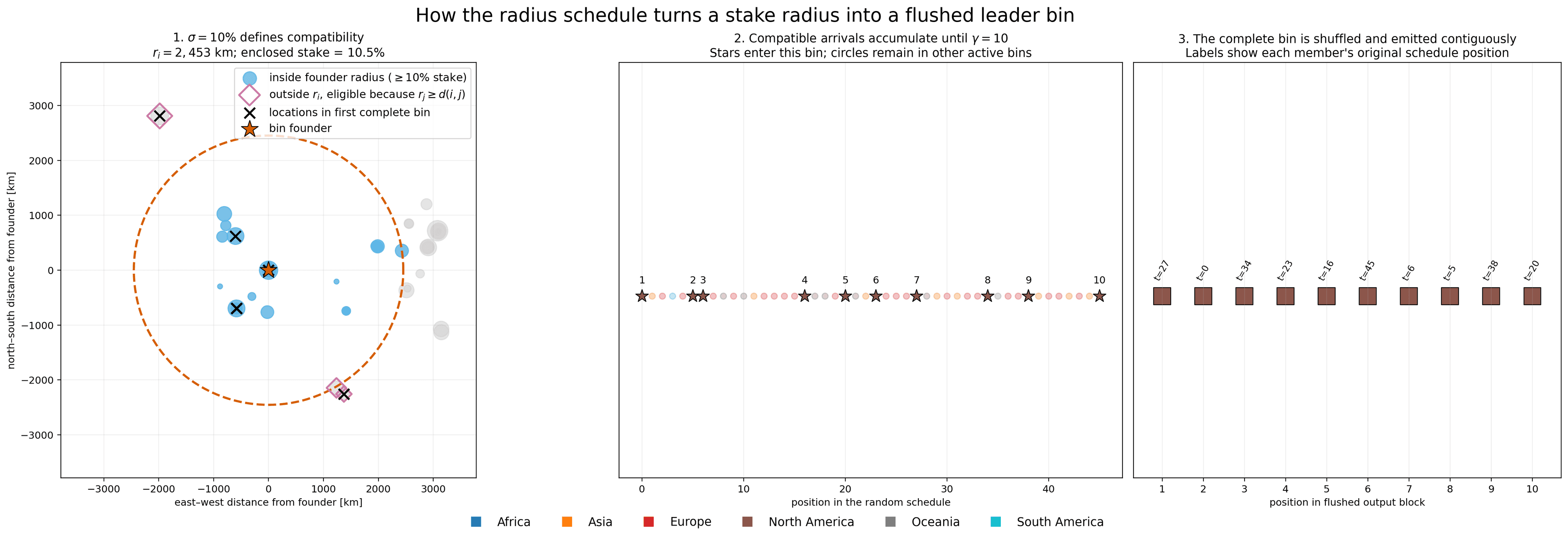
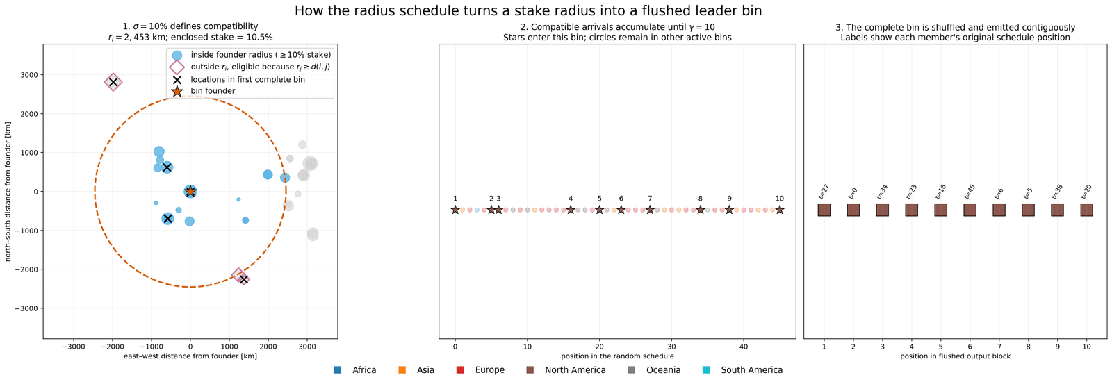
Left: the founder radius at and the areas suitable with it. Centre: suitable leaders accumulate within the bin till . Proper: the total bin is shuffled and emitted contiguously.
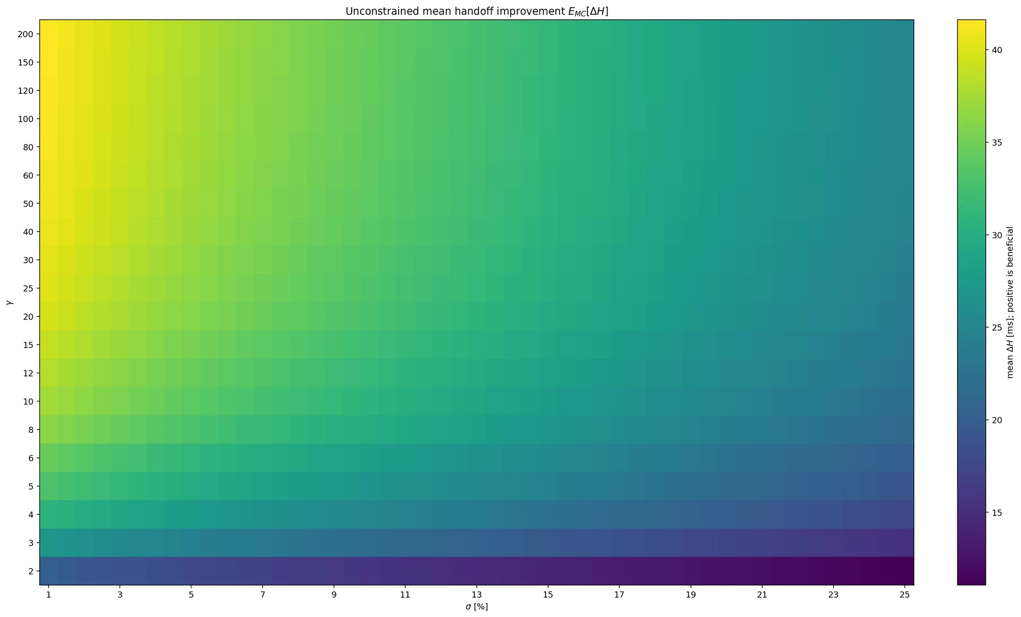
Imply handoff achieve throughout all artificial networks within the simulations, for each parameter choice.
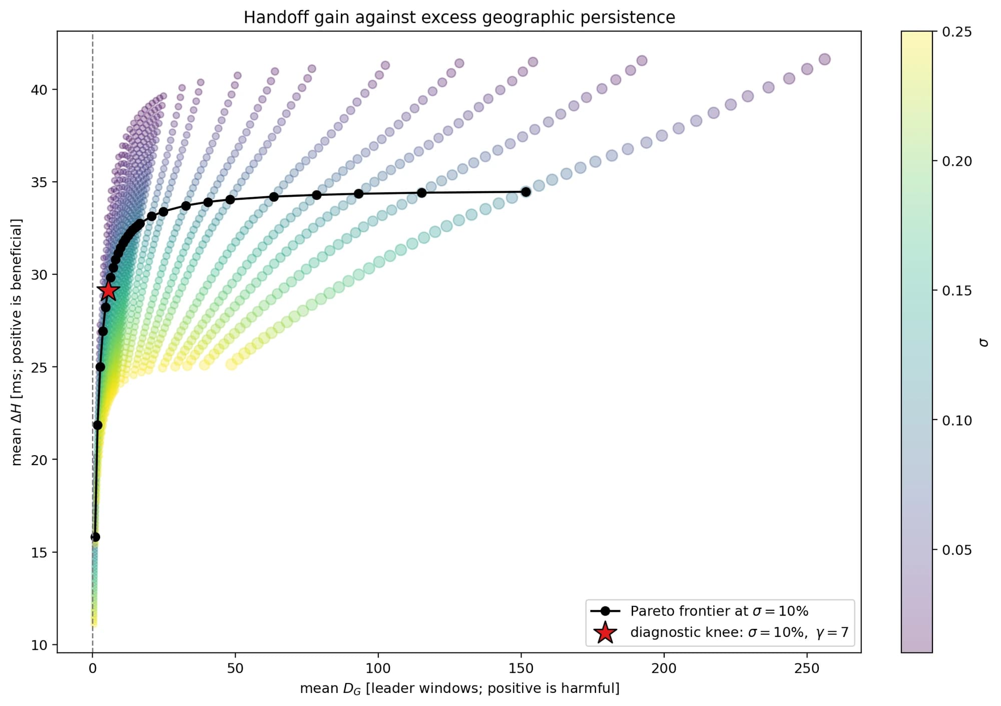
Imply handoff achieve towards imply extra geographic persistence , throughout artificial networks. Each simulated is proven, coloured by and sized by . The black line is the Pareto frontier at ; the star marks its knee, computed for .
Introduction
Solana’s chief schedule is what decides which validators are entitled to provide a slot.
The present schedule assigns home windows of 4 consecutive slots to every validator each epoch. The choice standards are primarily based on validators’ stake.
Regardless of being expensive to assault, a random schedule carries a well known situation: it ignores the place validators are positioned. Two consecutive leaders can sit in the identical information middle or on reverse sides of the planet. Within the second case, the handoff (passage from one chief to the opposite) prices tens of milliseconds of pure propagation delay.
SIMD-0675 proposes a geo-aware chief schedule. To be able to protect a number of the good properties of the random scheduler, the core extraction mechanism is just not changed. It takes the identical random schedule as enter and solely adjustments the order. Each validator retains precisely the identical variety of chief home windows it will have had.
The reordering is dependent upon two parameters (see Fig. 1):
- (
STAKE_FLOOR): For each location we compute a radius : the smallest distance that accommodates not less than a fraction of the overall stake. Dense areas get small radii, remoted validators get massive ones. Two leaders are suitable when their distance is inside the bigger of their two radii - (
RUN_LENGTH): We undergo the random schedule so as. Every chief joins a suitable open bin, chosen at random, or opens a brand new one. When a bin reaches leaders, it’s shuffled and written to the ultimate schedule as one contiguous block.
Fig. 1: Left: the founder radius at and the areas suitable with it. Centre: suitable leaders accumulate within the bin till . Proper: the total bin is shuffled and emitted contiguously.
The concept is easy: consecutive leaders change into geographically shut, so the handoff turns into shorter. However this comes at a worth: the ultimate ordering is transferring away from the random chief schedule.
The aim of this evaluation is to quantify the trade-off between latency achieve and assault floor enlargement, ultimately offering a information for parameter choice. Exactly, we attempt to reply the query: How a lot latency will we achieve for a given alternative of , and the way far does the schedule transfer from random to get it?
The evaluation is structured to first current all of the metrics employed. Within the second half we use the noticed behaviour to supply wise values for these parameters.
Related SIMDs are
The Parameter Choice Tradeoffs
Community state is consistently altering. Stake can redistribute, nodes can transfer round, new coalitions can kind. Thus, we will’t examine how parameters have an effect on at the moment’s community, however we have to add perturbations.
On this evaluation, we hold the 124 areas the place Solana validators run at the moment, grouped in six macroregions, and generate 6,250 artificial networks on high of them by redistributing nodes and stake with totally different ranges of focus (see Appendix A).
Because of the absence of proof of different websites able to host Solana nodes at the moment, we add no new areas to the simulation pipeline. The geography due to this fact stays as unbalanced as it’s now.
All conclusions are conditional on this geography. If new areas change into accessible within the smaller areas, or stake strikes considerably throughout areas, they need to be revisited.
Handoff Acquire
To be able to measure the latency enchancment, we make use of the handoff for a schedule outlined as the common latency between consecutive leaders,
the place is the overall variety of chief home windows within the simulations (108,000 right here), is the chief of window , and is the estimated latency between chief and chief . We estimate it from distance solely: , i.e. alerts journey in fiber at about two thirds of the velocity of sunshine alongside a path 50% longer than the great-circle distance.
The achieve over random is
so optimistic values imply the geo-aware schedule is quicker than random.
Fig. 2: Imply handoff achieve throughout all artificial networks within the simulations, for each parameter choice.
Determine 2 exhibits two clear traits. The achieve grows with and shrinks with . At , it goes from 15.8 ms at to 33.9 ms at . At fastened , transferring from to prices roughly a 3rd of the achieve.
This behaviour is predicted by the character of the parameters:
- A smaller means smaller radii, so leaders in the identical bin are nearer to one another
- In a block of leaders, handoffs are between suitable leaders and solely the final one jumps to the subsequent bin. The share of lengthy jumps is then roughly .
It’s fascinating to look at that, the second level explains why the achieve saturates. Going from to solely removes a small share of the lengthy jumps, and that share retains shrinking. At , already provides 65% of the achieve noticed at , provides 79%, and provides 91%. Past , every extra chief per bin buys little or no latency.
Geographic Persistence
The aim of a geo-aware schedule is to group chief from the identical space. Inevitably, because of this the community stays longer in a single macroregion. If that area has an issue, akin to an outage at a big supplier, native censorship or a regional community partition, the community is uncovered to it for longer than below random.
That is clearly decreasing the resilience of the community. Thus, we have to measure the “loss” we get after we change the parameters.
We measure the likelihood that consecutive chief home windows all fall in the identical macroregion,
the place is the macroregion of the chief . We measure extra cumulative geographic persistence relative to random as
For every , the beginning place is uniform over the legitimate positions. sums extra homogeneus-block possibilities throughout lengths. It measures cumulative geographical persistence.
It’s price mentioning that, additionally supplies a proxy for added time spent consecutively in the identical macroregion. For , and for suffciently bigger , the residual same-region length will be expressed as
the place represents the length of 1 chief window. Consequently, is expressed in chief home windows, and multiplying it by 0.8s provides a time-scaled persistence measure. All through the textual content and figures, references to extra home windows or seconds of geographic persistence use this approximate interpretation.
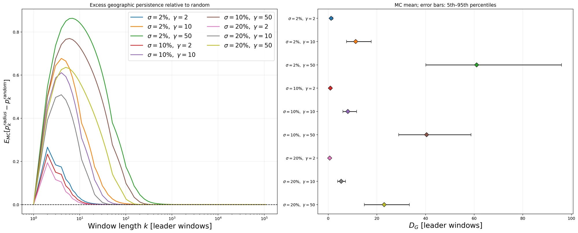
Fig. 3: Left: imply extra persistence as a operate of the window size (in chief home windows). Proper: , MC imply with fifth–ninety fifth percentiles throughout artificial networks.
The surplus peaks at quick horizons, just a few home windows, after which decays. Two issues management it.
- It’s clear that is the dominant issue. Bigger bins imply longer same-region blocks, so each the height and the tail develop. With the surplus is gone after about 20 home windows; with it lasts for just a few hundred
- Shifting reduces the surplus of geographic persistence. It is because a bigger provides bigger radii, so bins combine extra areas and extra areas. At , goes from about 61 home windows at to about 23 at , and the unfold throughout networks shrinks as effectively.
That is the primary trade-off. For the handoff, smaller and bigger are higher. For persistence, each are worse. Bigger bins purchase latency with longer stays in a single area, and smaller radii make these stays extra probably.
Regional Occupancy
Persistence counts uninterrupted runs. A single chief from one other area breaks a run, even when the community then goes again to the identical area. To seize how concentrated the schedule is over a complete interval, we take a look at the share of essentially the most represented macroregion in a window of consecutive chief home windows
Beneath random, each interval accommodates every area roughly in proportion to its stake. A curve shifted to the proper of random signifies that intervals are extra typically dominated by one area.
We use 4 horizons: 38, 375, 1,125 and a couple of,250 chief home windows. With 200 ms slots these are about 30 seconds, 5 minutes, quarter-hour and half-hour.
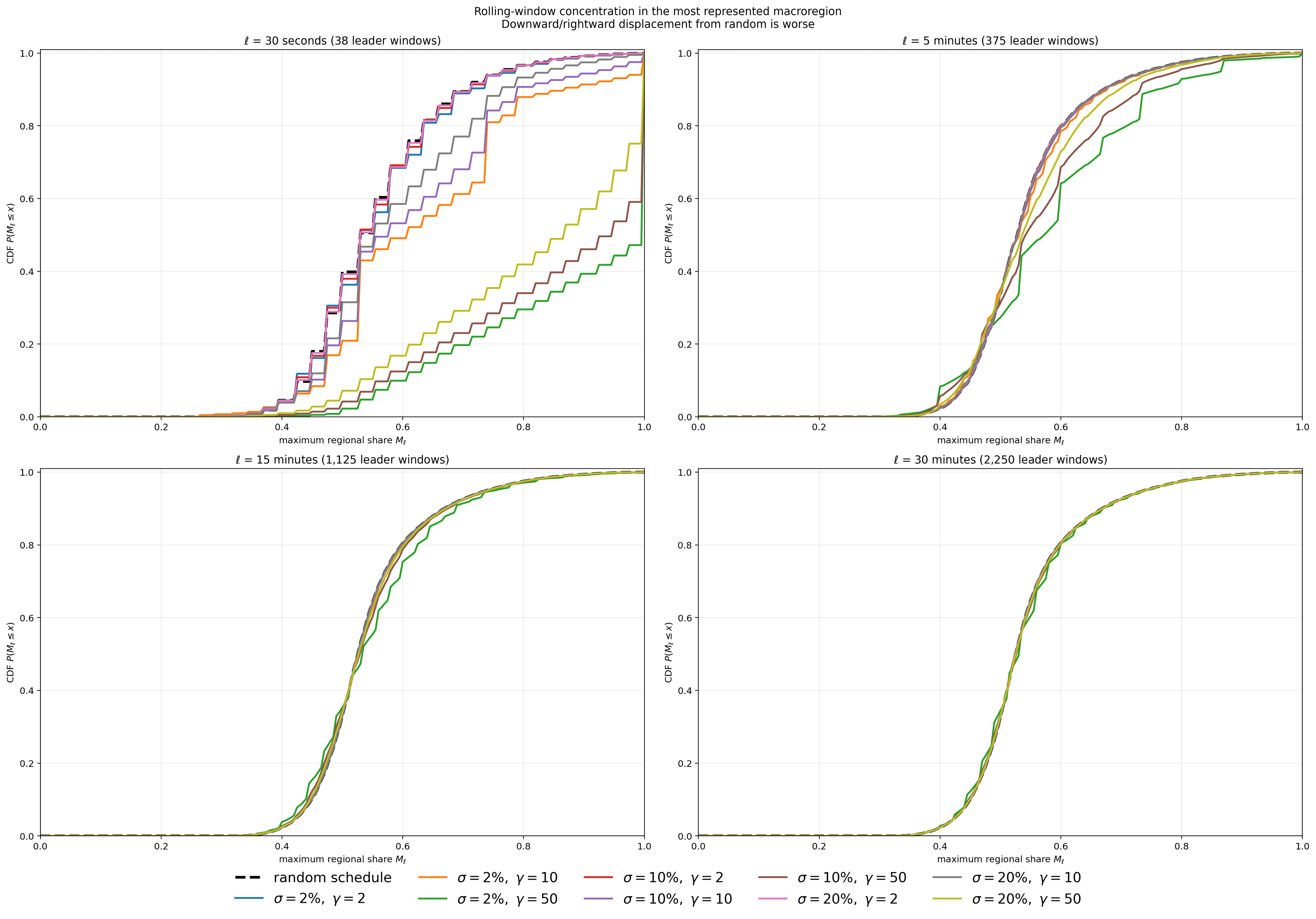
Fig. 4: CDF of the most important regional share over rolling intervals of chief home windows, for random (dashed) and chosen .
The primary message of Fig. 4 is that focus is a short-horizon impact.
- At 38 home windows (~30 s) the variations are massive. With the schedule is indistinguishable from random. With the curves transfer clearly to the proper. With a big fraction of intervals is dominated by a single area, for each . At , the imply extra of over random is 0.5 proportion factors at , 5.9 at and 29.5 at .
- At 2,250 home windows (~30 min) all configurations principally overlap with random.
This follows from how the schedule is constructed. The chief multiset is preserved and bins are flushed roughly within the order they fill. A pacesetter is moved solely by the point it takes its bin to fill. Over lengthy horizons the regional composition is due to this fact the identical as random; what adjustments is how areas are organized contained in the interval. As a substitute of being combined, they alternate in blocks.
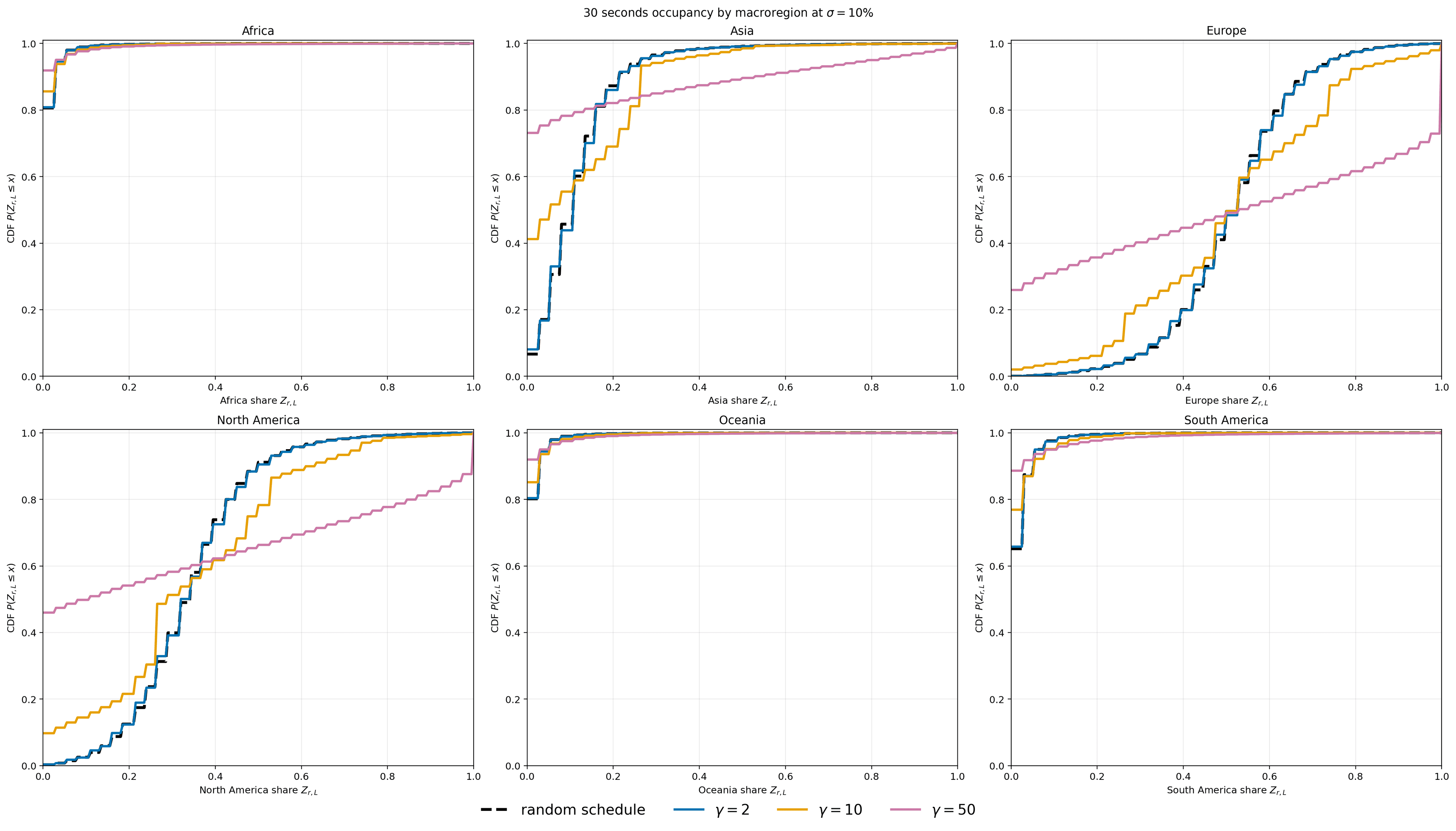
Fig. 5: Regional share over 38 chief home windows at , by macroregion.
Determine 5 exhibits who’s affected over quick horizons. In Europe and North America, bigger makes intervals extra excessive: with a few quarter of the 38-window intervals comprise no European chief, and roughly the identical share accommodates solely European leaders. Asia adjustments essentially the most in relative phrases. Beneath random, solely about 7% of those intervals haven’t any Asian chief; this rises to about 40% at and above 70% at . Africa, Oceania and South America barely transfer. Their leaders principally find yourself in bins based in different areas (see the spillover part), so they’re unfold out slightly than grouped.
The trade-off is identical as for persistence, however sharper. Quick-horizon focus grows shortly with , whereas many of the latency achieve is already reached at small .
Cross-Area Spillover
The radius is outlined by stake, not by geography. If a macroregion holds lower than a fraction of the overall stake, the radius of its areas has to achieve exterior the area to gather sufficient stake. Its bins then combine native and international leaders.
For bins based in macroregion , we measure the share of slots that belong to leaders from different areas,
The founder is at all times native, so can’t exceed .
Spillover is just not a danger with respect to random: a random block mixes areas much more. It tells us as a substitute the place the geo-aware schedule truly works. A area with excessive spillover will get little of the latency achieve, and its leaders are unfold inside different areas’ bins.
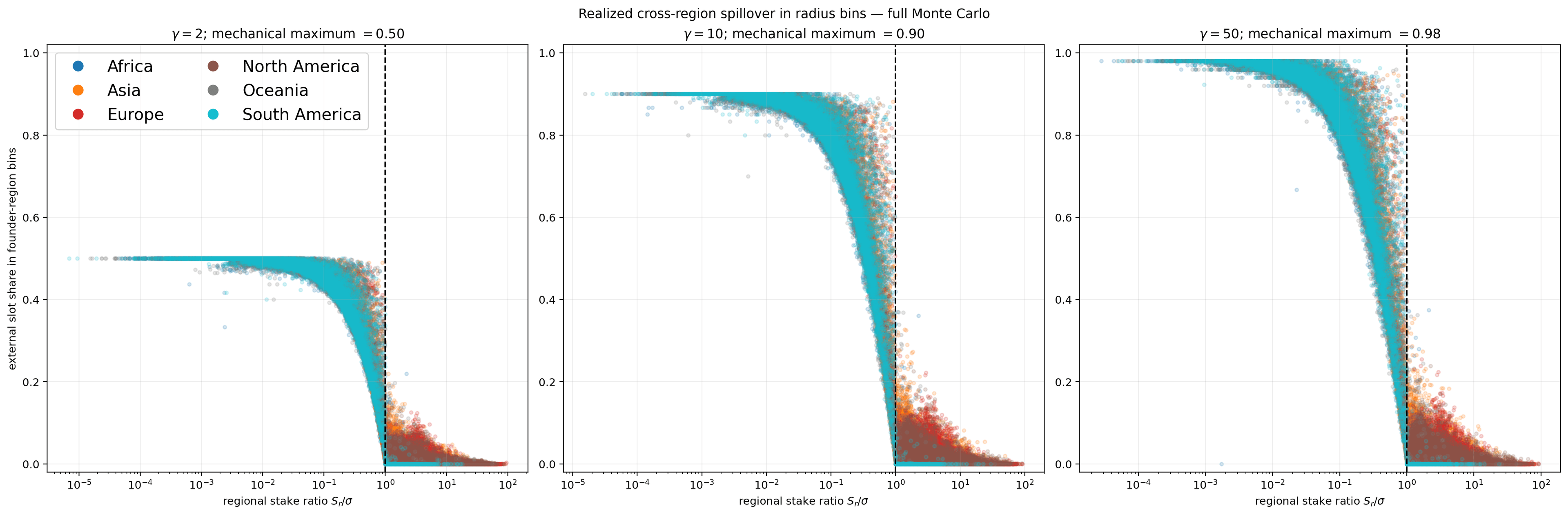
Fig. 6: Exterior slot share in bins based in every macroregion, towards the ratio between regional stake and . Every level is one area in a single artificial community. Dashed line: .
Determine 6 exhibits that one amount explains spillover: the ratio . All areas collapse onto the identical curve.
- When , bins are virtually self-contained. Spillover stays principally under 10% and reduces because the ratio grows.
- When , spillover rises steeply and shortly reaches its mechanical most. Bins based within the area are stuffed virtually totally by international leaders.
The transition is sharp and sits at . That is the explanation for an higher sure on : any area with much less stake than is successfully excluded from native bins.
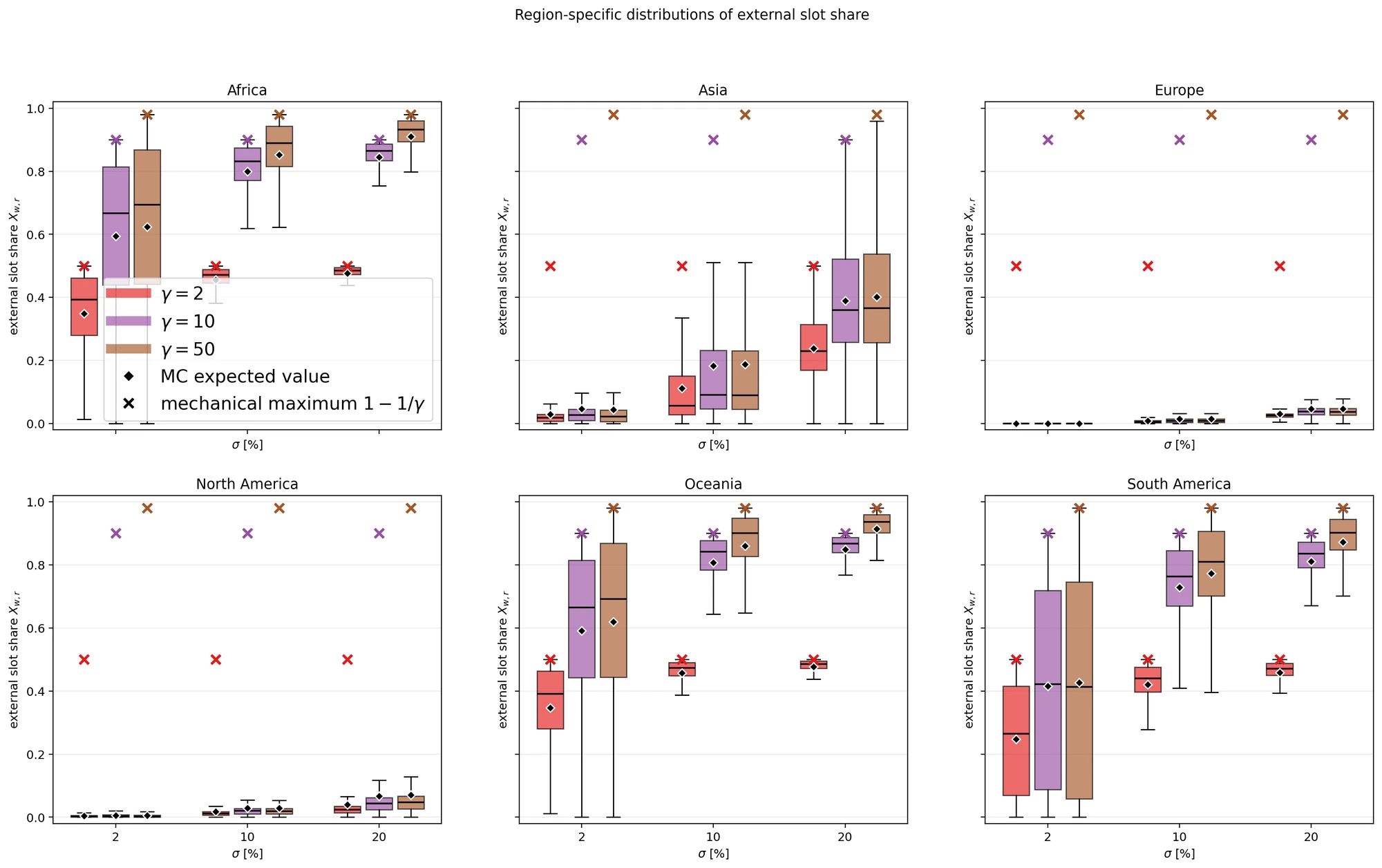
Fig. 7: Distribution of the exterior slot share throughout artificial networks, by macroregion, and . Crosses mark the mechanical most .
Determine 7 exhibits what this implies for every area below the present geography.
- Europe and North America are self-contained for each examined. Spillover stays at just a few p.c even at .
- Asia is the borderline case. At its bins are native. At the median is under 10%, however in some networks it reaches 50%. At its bins are principally combined. Asia’s stake share is about 11% on common throughout artificial networks and about 10.4% in at the moment’s snapshot, so sits slightly below it, with little or no margin.
- Africa, Oceania and South America have already got massive spillover at and are near the utmost at 10% and 20%. With one or two areas every, they maintain too little stake for any cheap .
Bigger will increase spillover in each area, as a result of a bin has extra slots to fill earlier than it’s emitted.
This provides the second facet of the trade-off on . Persistence and focus ask for a bigger . Spillover asks for a under the stake of the smallest area we wish to hold self-contained. Beneath at the moment’s geography that area is Asia, which places round 10%. This conclusion relies upon straight on how a lot stake Asia holds, and ought to be revisited if it adjustments.
Fictitious Location Assault
Validators declare their very own location, and the schedule trusts it. An actor that declares an remoted location can find yourself alone in its bins. Each full bin it fills turns into a block of consecutive chief home windows below its management.
If the stake declared at a location is not less than , the radius of that location is zero. An sincere chief can then be part of one among its bins provided that its personal radius reaches it, . In at the moment’s snapshot, an actor with 10% of stake on the remoted coordinate, within the South Pacific, at about , with , can be reachable solely by validators in a single Argentinian and one Australian location, holding collectively about 0.03% of the stake. Their radius reaches the actor exactly as a result of the actor’s personal stake is the closest 10% they will discover. In observe, its bins would comprise solely its personal home windows.
In a random schedule, a given block of consecutive home windows belongs totally to the attacker with likelihood . With and that is : it primarily by no means occurs.
We’ve already seen that growing concentrates future in the identical macroregion. That is logically true for single attacker of stake .
What we wish to measure now could be the achieve when the attacker declare a fictitious location. Exactly, we contemplate an attacker who controls a complete stake and declares a single coordinate so far as potential from each noticed location. Trustworthy stake is rescaled to .
For every simulated world, comparisons use the identical attacker stake (X) and the identical baseline chief schedule.
Let point out attacker management of chief window . Select uniformly amongst attacker-controlled home windows. Outline
That is the remaining consecutive management from the chosen window, together with that window.
For every world we will outline
and
the place ranges over the sampled truthful areas. Each metrics are measured in chief home windows; reported means subsequently common throughout Monte Carlo worlds.
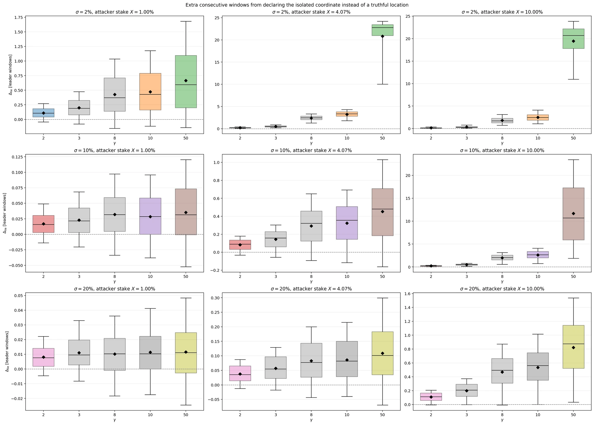
Fig. 8: Acquire from mendacity concerning the location. Containers span the interquartile vary, the road is the median, whiskers are the fifth and ninety fifth percentiles and diamonds the imply. Vertical scales differ between panels. Damaging values imply the truthful location already yields longer runs than the remoted coordinate.
Determine 8 exhibits how the safety threshold is dependent upon the attacker’s stake. If the achieve in anticipated slots begins to extend. It follows that such a assault is discouraged when is as excessive as potential.
It’s price noting that, an excessive worth of as soon as is fastened tends to augument the good points of mendacity concerning the place.
Pareto Frontier and Geometrical Tradeoff
At this level, we have now to look at that there isn’t a configuration that maximizes the handoff achieve and minimizes each danger directly. Nevertheless, the evaluation accomplished to this point may help us select the 2 parameters.
Selecting the Stake Ground
Nearly each danger we measured decreases as grows: persistence, short-horizon occupancy, bin dominance and coalition persistence. Solely two issues push the opposite approach. The handoff achieve is bigger for small , and spillover units a tough ceiling: as quickly as a area holds lower than of the stake, its bins cease being native (Fig. 6).
Nevertheless, we have now seen that can also be controlling the dimensions of the stake incentivized to misreport remoted coordinates. Thus, greater is greater is the stake wanted to achieve the inducement. In different phrases, you need to be as excessive as potential.
The tradeoff is then deciding on the very best worth of such that the smallest area with native bins at the moment preserves the locality.
The smallest area with native bins at the moment is Asia. Its stake share moved between 10.4% and 11.6% over epochs 1000–1041, and sits at 10.4% within the newest one.
We take the most important under that ceiling,
The worth is latency: at , the imply achieve is 29.8 ms at towards 35.4 ms at . In change, each safety metric improves. The margin to Asia’s stake is small, so this worth must be revisited if Asia’s share drops.
Selecting the Run Size
With fastened, each the achieve and the dangers develop with . Among the many dangers, regional occupancy issues little for this alternative: over 5 minutes it’s already indistinguishable from random for , and over quarter-hour for each , whereas outages sometimes last more than that. What actually adjustments is how lengthy the community stays in a single area with out interruption.
Since achieve and danger develop collectively, virtually each worth of at sits on the Pareto frontier. To seek out the place the trade-off turns, we use the knee: the purpose that maximizes the normalized achieve minus the normalized danger, measured from the random schedule to . Bigger values of are proven, however aren’t candidates for the knee, as a result of bigger bins purchase virtually no latency.
Fig. 9: Imply handoff achieve towards imply extra geographic persistence , throughout artificial networks. Each simulated is proven, coloured by sigma and sized by . The black line is the Pareto frontier at ; the star marks its knee, computed for .
Determine 9 exhibits the 2 curves behave very otherwise. The achieve saturates shortly, whereas retains rising virtually linearly with . The frontier is steep for small and flat for giant .
The knee is at . There the schedule good points 29.1 ms, 86% of the achieve at , and has a imply cumulative persistence rating of 5.4 further home windows (4.3 s) on common. Past that time latency turns into costly. Going from to provides 1.7 ms for two.7 further home windows; going to provides 4.8 ms for 35 further home windows. The tail of same-region runs provides virtually the identical reply: its knee is at , on a grid that doesn’t embrace .
It’s price mentioning that, the knee is dependent upon the most important it sees: normalizing on as a substitute of strikes it to , solely as a result of the far finish of the frontier is pushed additional out.
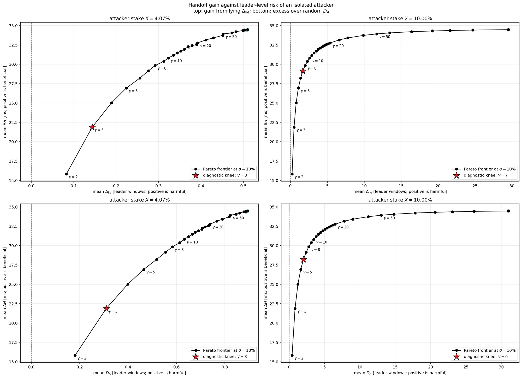
Fig. 10: Imply handoff achieve towards the leader-level dangers of an remoted attacker, at . Prime: achieve from mendacity concerning the location, . Backside: improve in anticipated remaining consecutive management, conditional on an attacker-controlled beginning window, relative to random, . Left: attacker with the most important stake at the moment, . Proper: attacker on the stake ground, . The black line is the Pareto frontier; the star marks its knee, computed for .
In Fig. 10 we report the Pareto frontier and relative knee evaluating imply handoff towards the leader-level dangers of an remoted attacker, fixing .
The knee solely describes the form of the frontier, not the extent of the danger. At , mendacity is price 0.28 home windows to an attacker with 4.07% of stake, and 1.69 home windows to an attacker with 10%.
Each knee falls between and . A price round sits on the knee of the regional dangers and of an attacker on the stake ground, and retains 86% of the achievable achieve. A price represents the conservative alternative if the precedence is the publicity to single validators under : it retains 65% of the achieve.
Related outcomes maintain below a second alternative of priors for regional stake displacement. With the regional stake prior of Appendix B, the place any macroregion can maintain the most important share of stake, the knee towards stays at and the knees for an attacker at are at for each dangers. For an attacker under , the knee towards stays at and the one towards strikes to , the place the danger is simply 0.03 home windows.
Pricing Each Millisecond
Up to now we have now chosen the parameters via knees. That works for , a lot much less for .
When reasoning about , we have now that it’s boxed in from either side. It must be bigger than the stake of any actor that would revenue from a fictitious location, and smaller than the stake of the smallest macroregion we wish to hold native. As we speak these bounds go away a slim vary round 10%.
The parameter doesn’t share the identical function. The dangers develop steadily with , whereas the achieve of every further step shrinks shortly, so the frontiers haven’t any pure break level. The knee we used solely seems as soon as we decide an finish for the frontier: with the most important at 20, 50 or 200, the knee towards falls at , 7 or 14. Any single worth of learn off a knee is due to this fact partly a product of the grid.
As a substitute of fixing parameters, we will present what every millisecond of handoff achieve prices, and let the reader resolve how a lot danger a millisecond is price.
All dangers on this evaluation are counted in chief home windows: further consecutive home windows in the identical macroregion (), or held by an attacker (, ). One window is 4 200 ms slots, so every danger converts on to milliseconds. For each and each step we then compute
the milliseconds of danger paid for every millisecond of handoff achieve. Step one begins from the random schedule, the place each are zero.
The 2 milliseconds aren’t the identical factor. A millisecond of handoff achieve is saved at each change of chief, i.e. each 0.8 s. A millisecond of danger is an anticipated stretch of time spent in a single area or below one chief. The worth tells us how briskly one grows in contrast with the opposite, not that they’re price the identical.
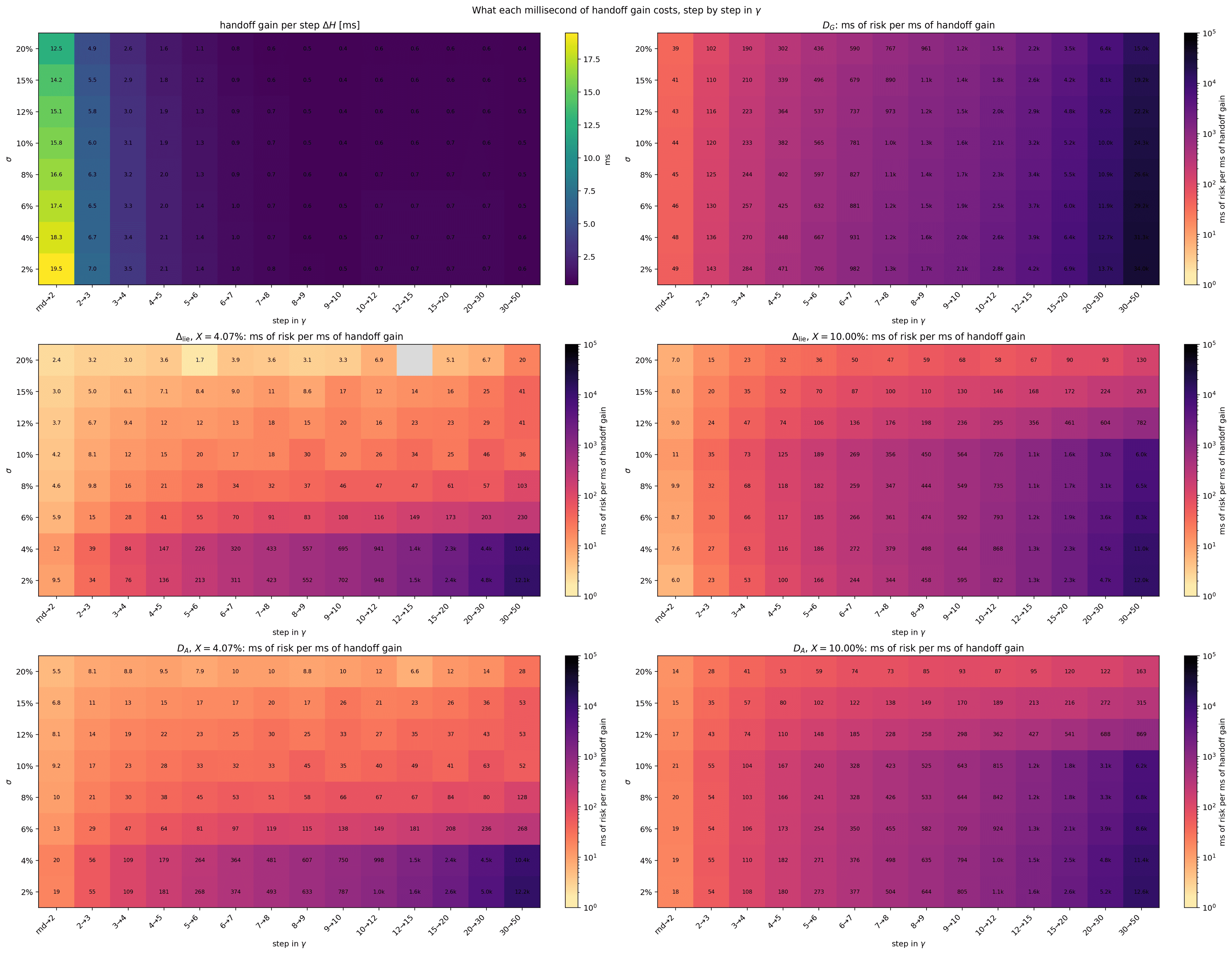
Fig. 11: Prime left: handoff achieve of every step in by . Different panels: milliseconds of danger paid for every millisecond of handoff achieve, for , and for and with an attacker at (the most important validator at the moment) and . Log shade scale; gray cells are steps the place the danger doesn’t develop.
The end in Fig. 11 turns the selection of into two easy questions: which danger will we care about most, and what’s the highest worth we settle for for a millisecond?
As soon as the worth of a step goes above that restrict, each later step prices much more. Going additional isn’t rational for that precedence, so the restrict units a most .
Particularly, represents a candidate compromise, not a preference-independent optimum. At 7 the achieve begin to saturate. Above 7, the geographic persistence prices 1s for each ms gained. If that is the utmost price we’re prepared to pay for further ms in handoffs, represents our most.
Under the selection is dependent upon the precedence. Accepting the common worth results in . A stricter worth results in a smaller : about 500 ms per ms for regional persistence provides , 250 ms per ms provides , and defending validators under provides .
The rational alternative is due to this fact a spread slightly than some extent. stays near 10%, fastened by the stake of the most important actors and the dimensions of the smallest native area. lies between 3 and seven, and the place it sits in that vary relies upon solely on the worth we placed on a millisecond of handoff.
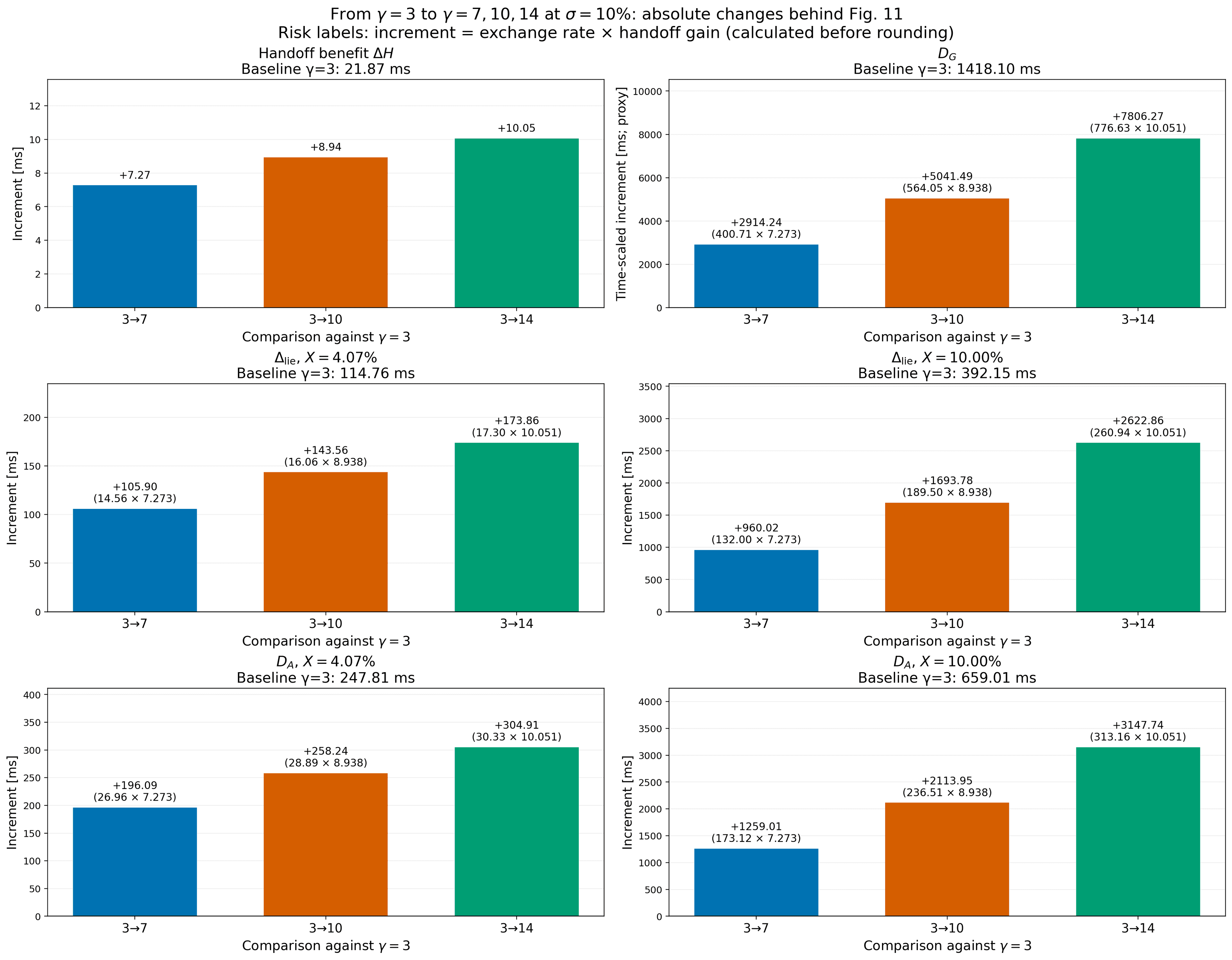
Fig. 12: Handoff enhancements and danger improve transferring from .
Appendix
Appendix A – MC Methodology
The core of this evaluation is to supply an evaluation of parameters implications that’s as a lot as potential unbiased from present community snapshots. It is because an evaluation accomplished over a set stake distribution dangers to introduce some dependencies on the peculiar configuration we measure at the moment.
Because of this we implement a MC simulation with the next prescription
-
We outline a factorial grid of Gini coefficients
-
For each Gini pair, we generate 250 unbiased community realizations, giving 6,250 artificial networks.
-
Uniform integer prior for variety of nodes in [400,2000]
-
Validator-location possibilities are generated from lognormal weights. Their dispersion is calibrated to the goal node Gini via
Validator are then allotted throughout the noticed geographical assist
- Validator stakes are generated independently utilizing the identical Gini-controlled lognormal building and normalized to sum to at least one.
At this level, for every realization we will extract a baseline schedule of slots, which is sampled proportional to stake (present model). We then examine each level into the MC below variations.
The rationale why we used a Gini coefficient construction for stake and node simulations is that stake and nodes are likely to cluster. Additional, low values of Gini may also accomodate extra uniform distributions. Few samples are displayed under.
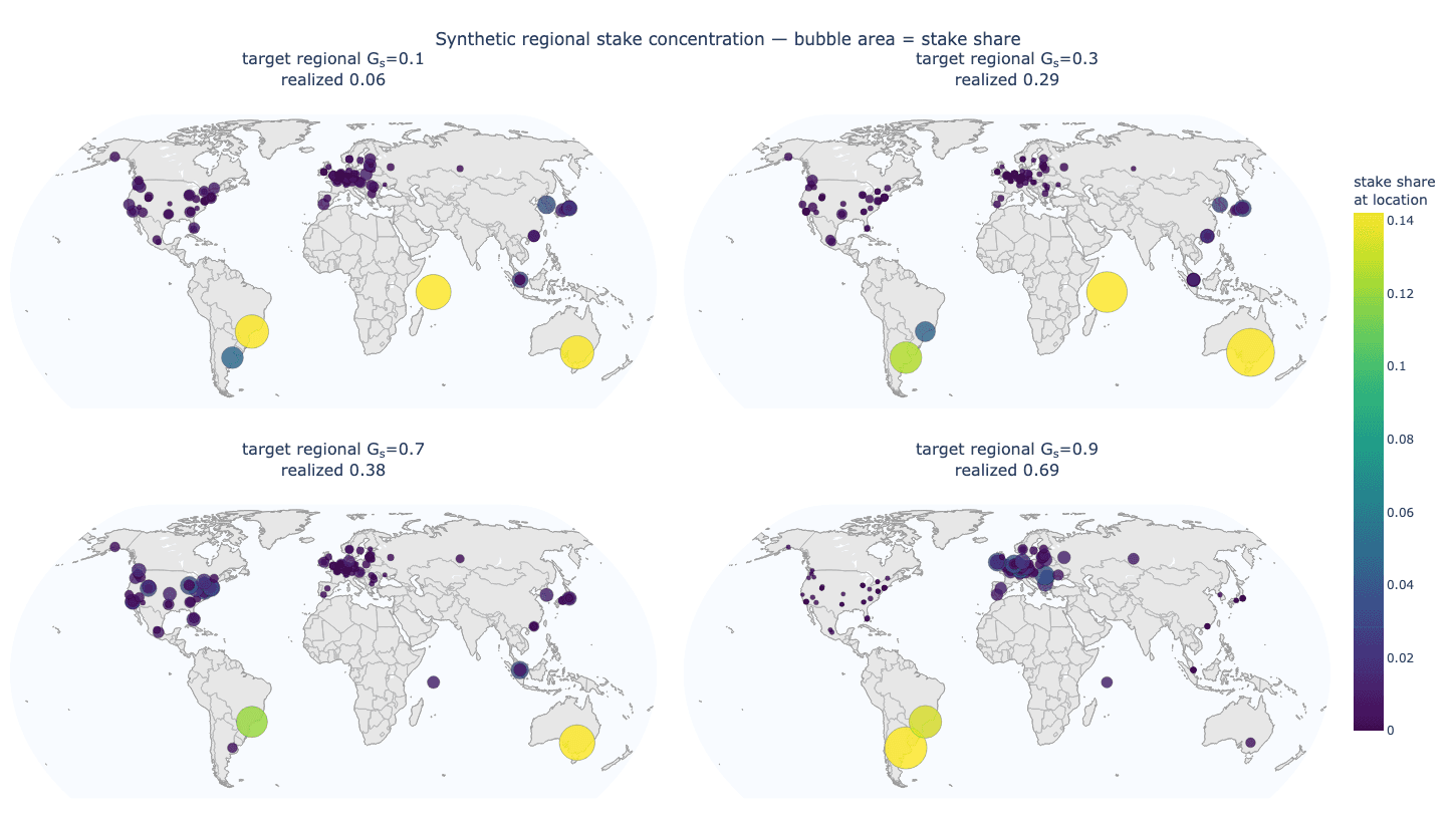
Fig. A1: Examples of regional stake distributions generated by the Gini priors for nodes and stake.
It’s price noting that, the usage of Gini doesn’t take away each dependence on the noticed snapshot. The geographical assist is fastened to 124 noticed areas and is very unbalanced throughout macroregions: Africa and Oceania comprise one assist level every, South America two, Asia fourteen, North America forty-two, and Europe sixty-four.
Since location weights are exchangeable throughout assist factors, anticipated regional mass is roughly proportional to the variety of accessible assist factors. The simulation due to this fact doesn’t mannequin new areas, regional enlargement, or migration past the noticed assist.
Additional, there’s a prior-sensitivity limitation. Regardless of the present snapshot, and node / stake evolution over time on each blockchain extremely justify the selection of priors, the reported outcomes may be prior-dependent.
All conclusions should due to this fact be interpreted as conditional on this generative mannequin. Specifically, the Monte Carlo can’t set up a parameter alternative that’s universally snapshot-independent.
Appendix B – A Random Stake Displacement
In the primary Monte Carlo, the stake of a macroregion roughly follows the variety of datacenters it hosts. Europe and North America maintain most of it, Asia sits round 10–11%, and Africa, Oceania and South America keep small in each community. Right here we drop that hyperlink and let stake transfer freely internationally.
The development is easy:
- each one of many 124 noticed areas hosts one validator, so the variety of nodes performs no position;
- the stake of every macroregion comes from lognormal weights calibrated to a goal Gini . The six weights are drawn independently, so any area can find yourself with the most important share;
- inside a macroregion, stake is cut up throughout its datacenters with a flat Dirichlet, i.e. each cut up is equally probably;
- coalitions are generated as in the primary evaluation.
Fig. B1: Examples of regional stake distributions generated by the Gini prior.
We generate 1,250 networks (5 stake Gini x 5 coalition Gini x 50 replicas), every with 108,000 chief home windows, and run a smaller grid of parameters:
- , plus for the frontiers;
- .
With solely six areas, the realized Gini falls under its goal, and the 2 most concentrated cells (0.7 and 0.9) find yourself very related. On this setup each area, Asia included, holds lower than 10% of the stake in about one community out of three.
The primary result’s that the image doesn’t change. The identical options that drive the primary evaluation are nonetheless there.
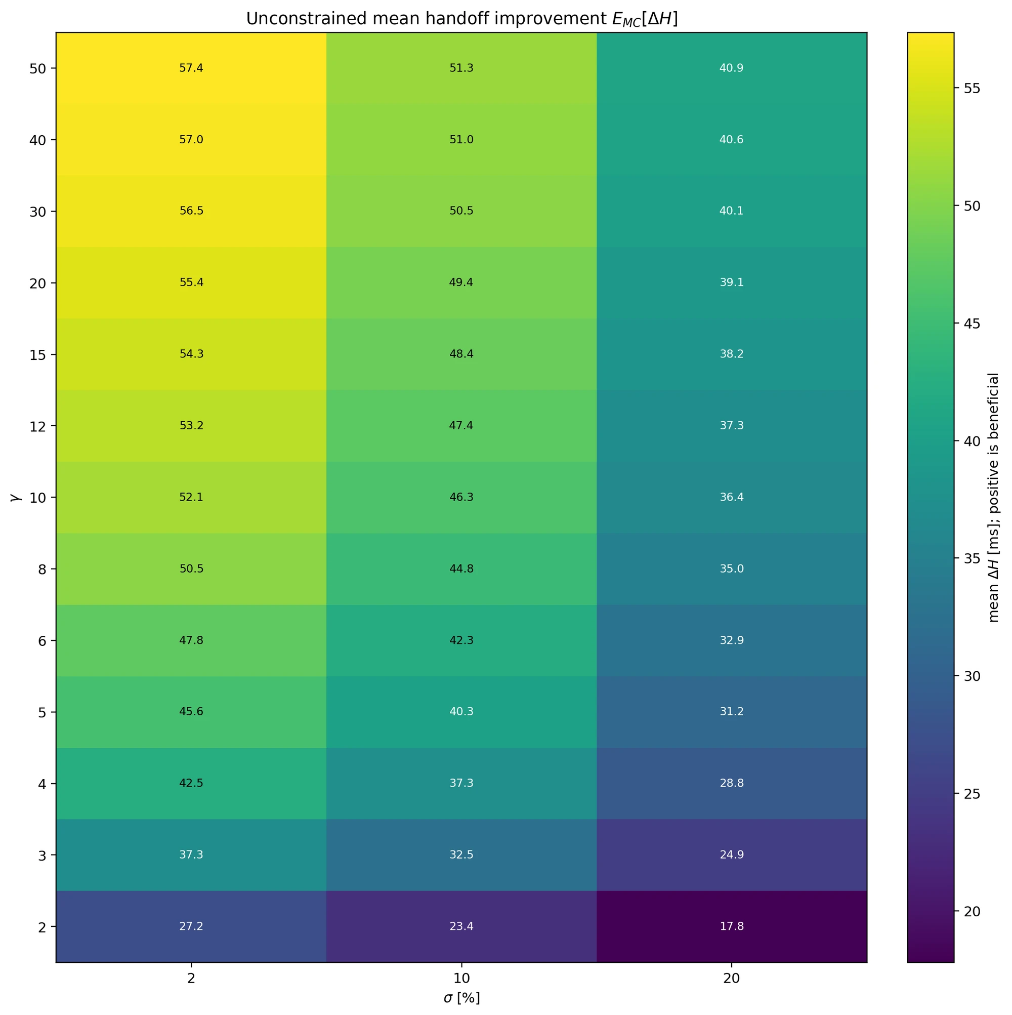
Fig. B2: Imply handoff achieve throughout all artificial networks within the simulations, for each parameter choice.
Handoff achieve and persistence behave as earlier than. Each develop with and the achieve saturates round . The achieve is bigger, as a result of with stake unfold throughout continents a random schedule jumps between areas extra typically.
Persistence is decrease: is 1.3, 5.7 and 26.7 home windows for a similar values of , towards 1.8, 8.1 and 40.4 in the primary evaluation.
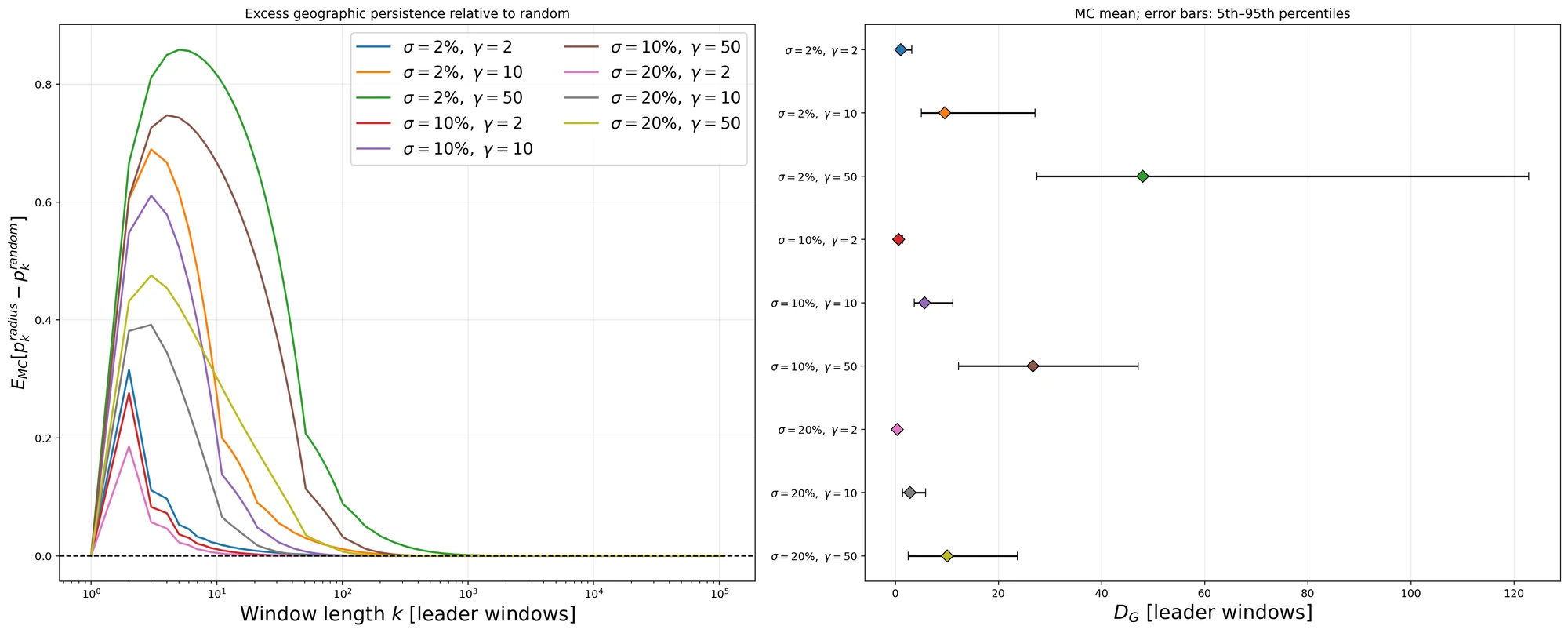
Fig. B3: Extra geographic persistence below the regional stake prior. Identical structure as Fig. 3.
Mendacity concerning the location nonetheless pays solely when the attacker’s stake approaches . At :
| Attacker stake | |||
|---|---|---|---|
| 1% | 0.00 | 0.00 | 0.00 |
| 4.07% | 0.02 | 0.05 | 0.09 |
| 10% | 0.56 | 3.0 | 16.0 |
Under the achieve is basically zero: for the median is about zero and in half of the circumstances the truthful location already provides longer runs. At the attacker good points a number of home windows, and the achieve grows shortly with . So nonetheless units the stake wanted to make the assault worthwhile, and a bigger nonetheless raises that bar.
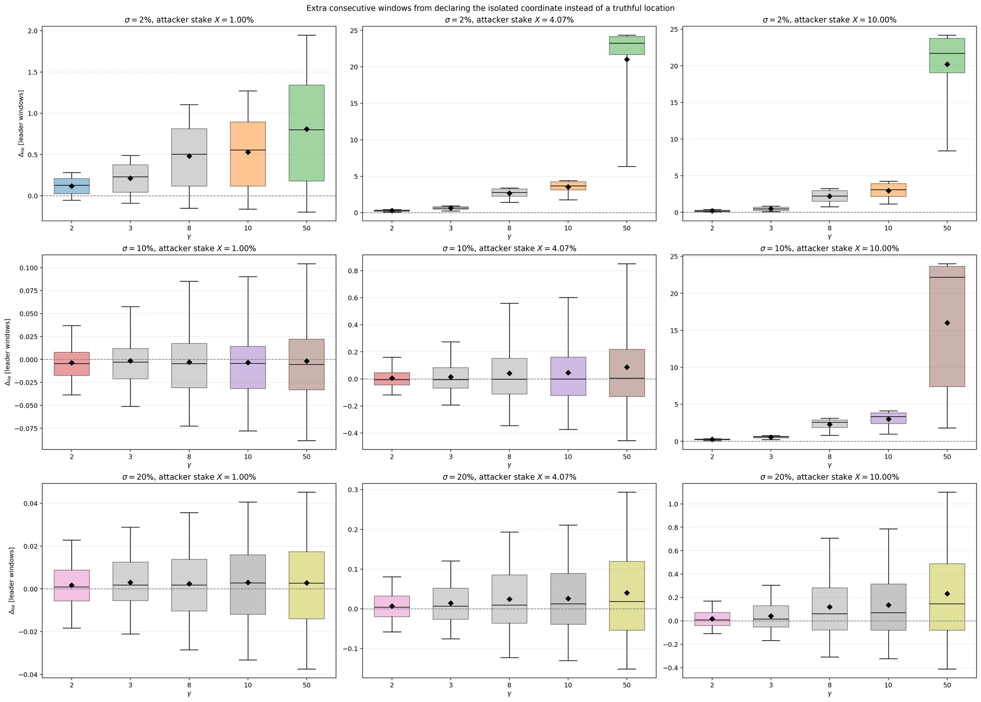
Fig. B4: Acquire from mendacity concerning the location below the regional stake prior. Identical structure as Fig. 8.
Spillover remains to be managed by the ratio . At any time when a area holds much less stake than , its bins fill with international leaders. Since this now occurs to each area in a few third of the networks, the tails attain excessive shares in every single place. At and the ninety fifth percentile of the exterior slot share is 0.86–0.88 in each area, towards a mechanical most of 0.90.
What adjustments from one area to a different is geography. On the similar ratio , Asia’s bins combine greater than the others. When Asia holds between half and three quarters of , the median exterior share of its bins is 0.63, towards 0.27–0.34 within the different areas. Asia’s 14 datacenters are unfold over hundreds of kilometers, from Japan to India, and sit near Europe and Oceania. Their radius reaches international stake earlier than it has collected sufficient Asian stake. Europe suffers barely, along with Oceania: their imply exterior share at and is 0.21, towards 0.25 for Asia and 0.18–0.20 for the opposite areas.
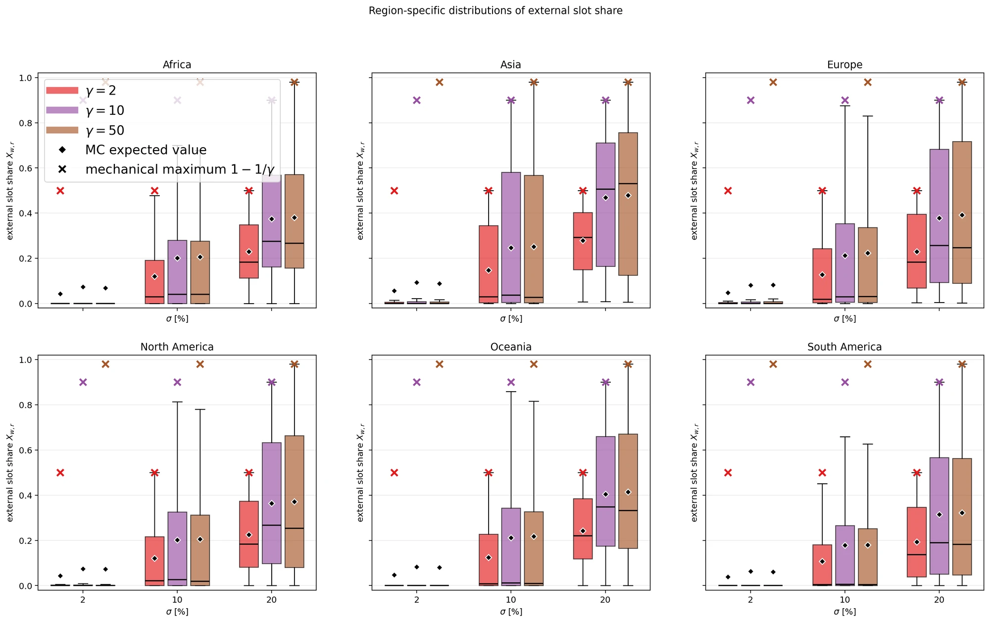
Fig. B5: Exterior slot share by macroregion below the regional stake prior. Identical structure as Fig. 7.
As in the primary evaluation, going past breaks the locality of the macroregions, ranging from Asia.
With , the knees on regional metrics don’t transfer. The knee of the handoff achieve towards stays at .
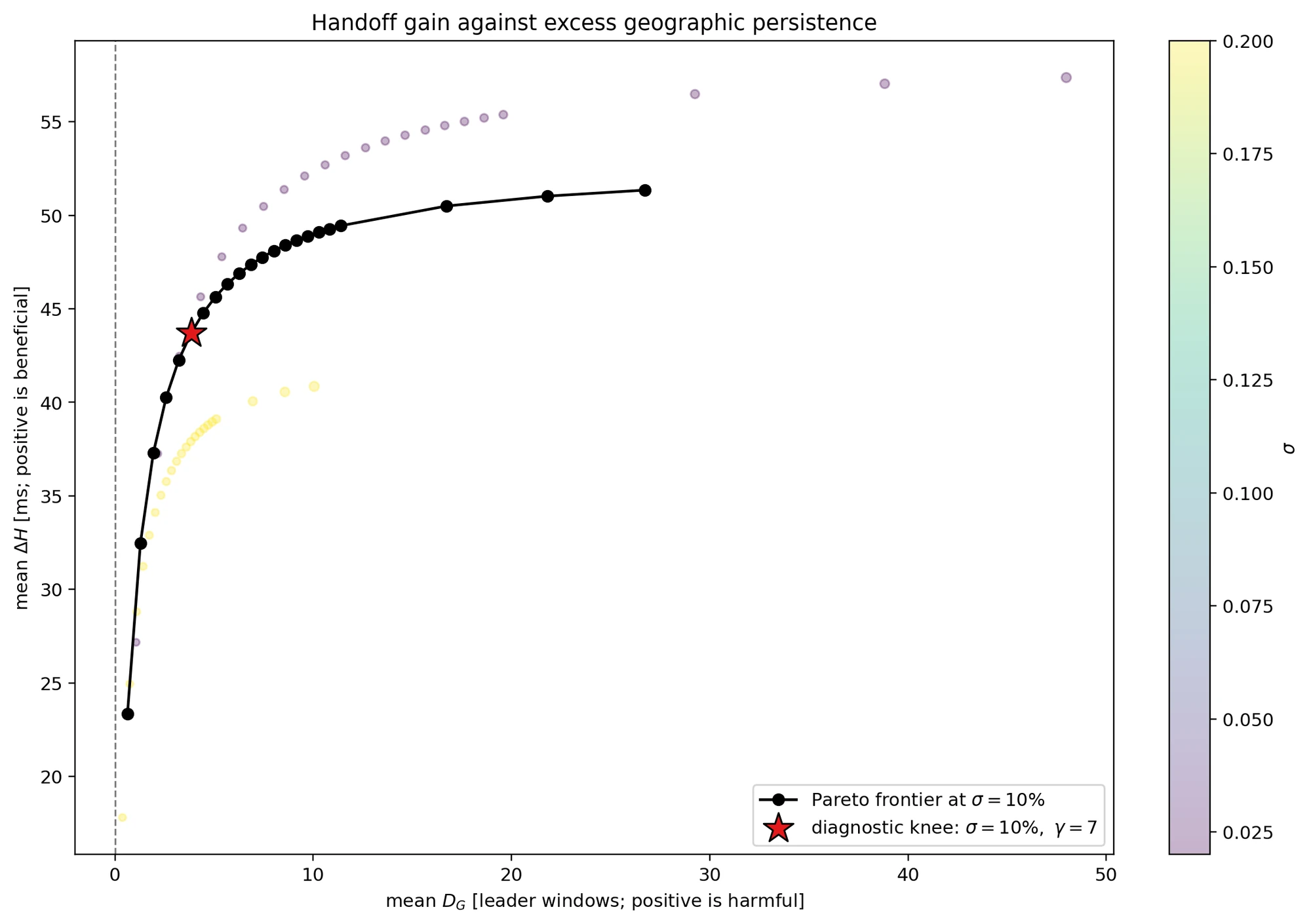
Fig. B6: Handoff achieve towards below the regional stake prior. Identical structure as Fig. 9.
For the leader-level dangers the image is analogous. With an attacker at , the knee is at for each and (7 and 6 in the primary evaluation). With an attacker under (), the knee towards strikes barely up, from to , whereas the knee towards stays at . On this case is tiny (0.03 home windows at ), so the precise place of its knee carries little weight.
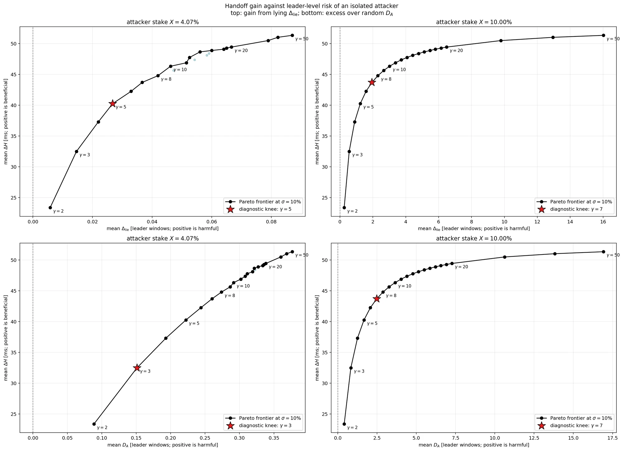
Fig. B7: Handoff achieve towards the leader-level dangers, (high) and (backside), for and , below the regional stake prior. Identical structure as Fig. 10.
A extra uniform and extra cellular stake due to this fact preserves the primary conclusions. Rising is reduces the measured profit from misreporting. Geography nonetheless caps round 10%, and at the selection of primarily based on the knees is basically unchanged.
Appendix C – Coalitions and Consecutive Slots
We will introduce the presence of coalitions and ask how the likelihood of acquiring consecutive home windows adjustments when transferring into geo-aware parameter house.
For coalitions right here we confer with any kind of collaboration between teams of validators. We use the identical Gini-based simulation pipeline. Gini coefficients for coalition are within the set . It is because coalitions often give incentives, and validators often choose in into coalitions that pay essentially the most.
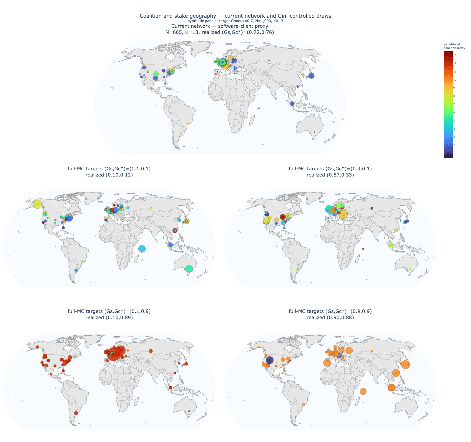
Fig. C1: Examples of regional coalitions distributions generated by the Gini prior.
At this level we will examine the surplus likelihood with respect to random of proposing consecutive home windows.
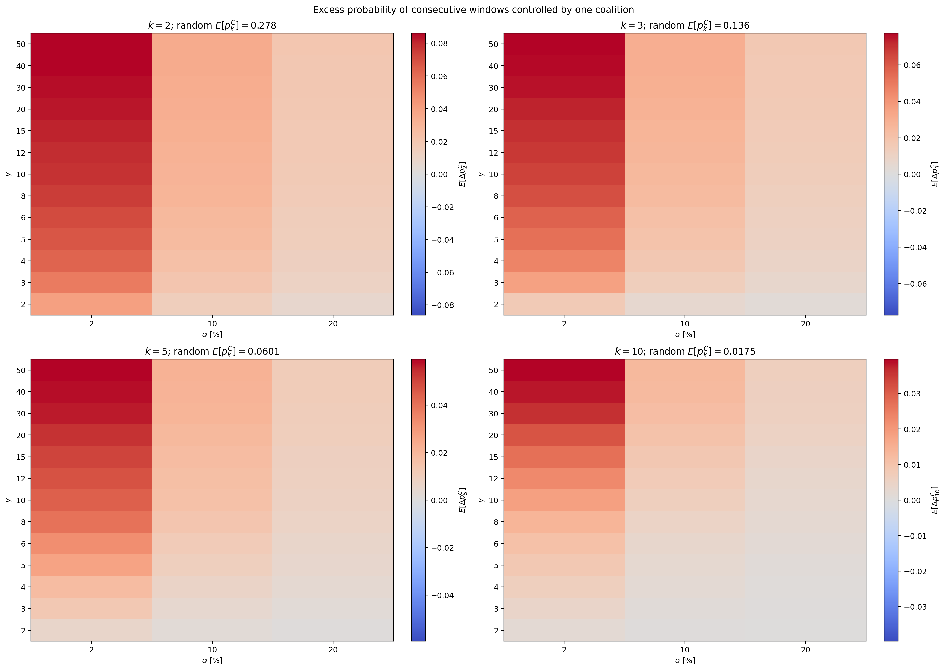
Fig. C2: Extra likelihood (with respect to random schedule) of acquiring 2, 3, 5, 10 consecutive home windows.
Determine C2 exhibits how this likelihood adjustments. When fixing , we have now
| chief home windows | |||
|---|---|---|---|
| 2 | 29,83% | 30,72% (+0,89 pp) | 30,84% (+1,01 pp) |
| 3 | 14,85% | 15,93% (+1,08 pp) | 16,07% (+1,22 pp) |
| 5 | 6,46% | 7,43% (+0,97 pp) | 7,59% (+1,14 pp) |
| 10 | 1,86% | 2,23% (+0,37 pp) | 2,38% (+0,52 pp) |
We observe that absolutely the increments stay restricted within the configurations thought-about. At , the likelihood that three consecutive chief home windows belong to the identical coalition strikes from roughly 14.85% at to 16.07% at . For 10 consecutive home windows, it strikes from 1.86% to 2.38%: a relative improve of roughly 28%, however an absolute improve of 0.52 proportion factors.
That is related when assessing extra alternatives for coalition-based MEV. The radius schedule preserves every coalition’s whole variety of chief home windows however adjustments their temporal association. In these simulations, growing produces a restricted absolute improve in consecutive coalition management. Nevertheless, this doesn’t straight quantify extra MEV income.
Appendix D – Sensitivity to incorrect geographical coordinates
Incorrect coordinates can come up from deliberate misreporting or operational adjustments, akin to relocating a validator with out updating its declared place. We assess this mismatch utilizing an artificial validator holding stake fraction . Scheduling makes use of declared coordinates, whereas outcomes are evaluated at bodily areas.
For every metric, reference schedule and parameter configuration, we choose a declared coordinate that maximizes the frequency of decay on coaching networks, then consider it on separate validation networks. Determine D1 stories
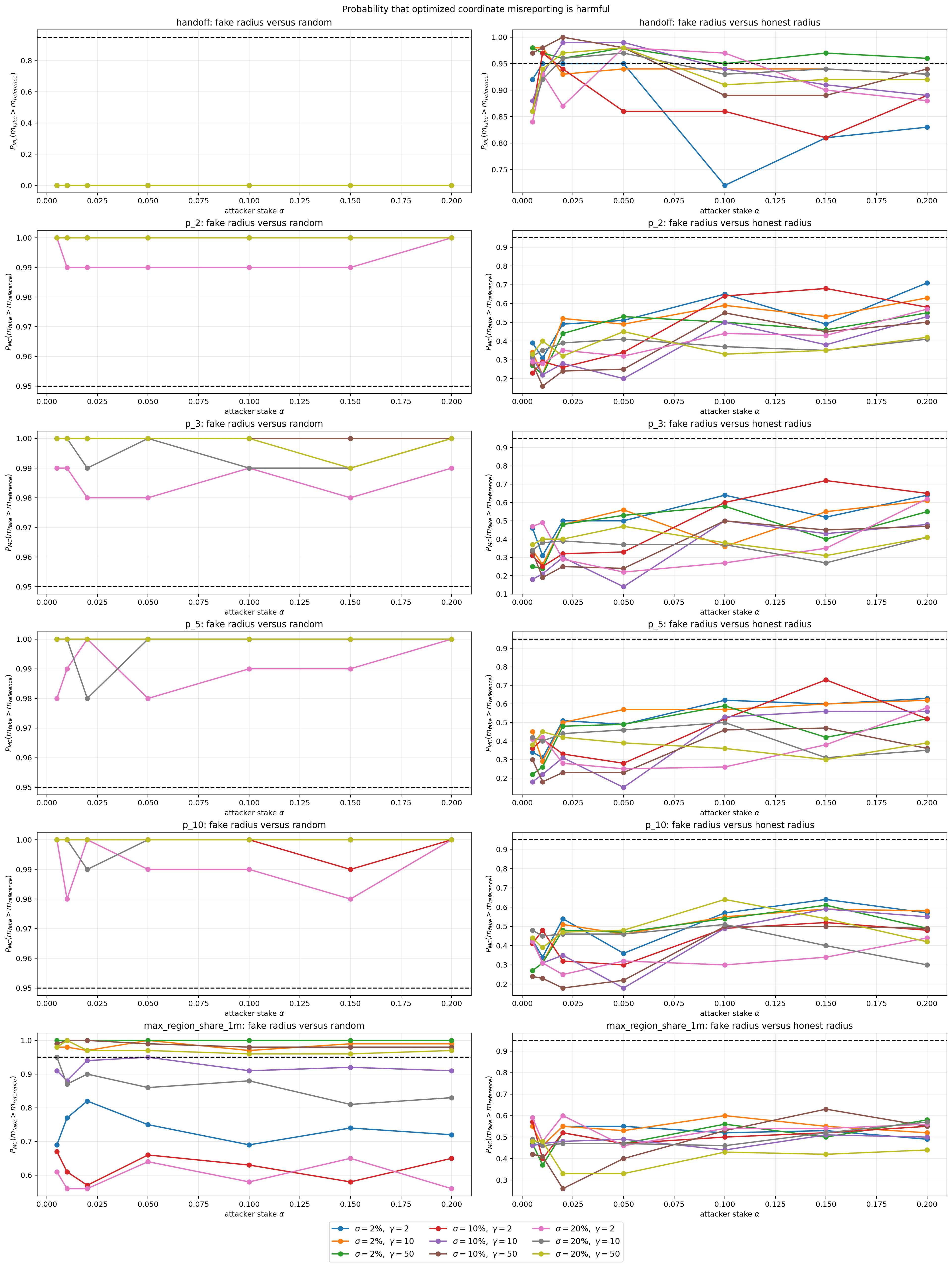
Fig. D1: Sensitivity to optimized coordinate misreporting. Every curve exhibits the fraction of validation networks through which incorrect coordinates improve the metric indicated by the row, relative to random scheduling (left) or accurately reported radius scheduling (proper). The horizontal axis provides the stake fraction assigned to the misreporting validator; colours establish . Rows report imply handoff latency, same-macroregion persistence for consecutive chief home windows, and imply most regional occupancy over one-minute intervals. Declared coordinates are chosen individually for every metric, reference and parameter configuration on coaching networks, then held fastened throughout validation. All outcomes use bodily areas. The dashed line marks a 95% frequency of decay, not a confidence interval. Possibilities describe the frequency, not the magnitude, of decay.
Columns evaluate towards random scheduling and accurately reported radius scheduling. The dashed line marks 95%, not a confidence interval.
Misreporting ceaselessly will increase imply handoff relative to accurately reported radius scheduling. Nonetheless, no handoff deterioration relative to random is noticed within the displayed validation outcomes, even at .
Geographic persistence is sort of at all times greater than below random scheduling. Nevertheless, its extra deterioration relative to accurately reported radius scheduling is much less constant. The identical distinction applies to imply most regional occupancy over one-minute intervals. Thus, comparability with random contains the clustering already launched by the radius algorithm; it doesn’t isolate the impact of incorrect coordinates.
These curves measure how typically deterioration happens, not its magnitude. They describe an adversarially chosen coordinate-mismatch stress check, slightly than the anticipated influence of routine relocations.

